Mathematical optimisation is the branch of mathematics that using a set of techniques and algorithms aims to select the best elements of a group (concerning some criterion), subject – or not – to requirements formulated in terms of constraints.
Since the dawn of civilisation, the human species has searched for ways to find the best way to achieve a goal. For example, the best way to transport goods, or the quickest, to get from point A to point B.
Increasingly, companies realise the potential of mathematical optimization to improve their business. For example, a petrol supply company is interested in knowing the best place to place its dispensers, or a transport company can find out how many trucks are needed to satisfy the demand for their products and avoid, in this way, the loss of sales. However, theoretical and practical knowledge of these techniques is necessary for applying them successfully. In addition, the problem is often not well defined and presents complex challenges when it has to be solved.
This article will present the basic concepts that define an optimisation problem. We discuss the three steps for obtaining the optimum: understanding the needs of the client, constructing the problem and solving it. We will also explain the difficulties that may arise and the good practices to follow. Finally, we will present some examples of software and libraries that help us solve optimisation problems.
Structure of an Optimisation Problem
To successfully classify and solve an optimisation problem, it is first necessary to identify the three key pieces that make up the problem:
- What is the decision: Before any model is proposed, we need to be clear about the decisions and what can be done in the system to make it work “better”. For example, if it is about supply chain management, do you decide only what the flows will be or where to locate the facilities? In the first case, only the best quantity of each product family to be transported between the different facilities will be obtained. In the second case, the amounts transported and where the facilities will be located from a set of possible candidate locations will also be obtained.
- Requirements: We have to understand what elements and restrictions the problem has, as generally speaking, the limitation of resources will limit the range (set) of possible solutions. For example, we will have to deliver a quantity equal to the demand for each family of products and clients.
- Indicator to optimise, for which we want to find the optimal value. For example, the total cost of the operation, the supply chain or the quality of service. This indicator is also known as the objective function or cost function.
Sometimes the problem will be straightforward and the pieces will be easy to model. In other cases, one or more of the above points will be difficult. Generally, the problem will be more difficult at most points. It should be approached staggered, first by posing small, simpler subproblems and gradually increasing their difficulty as they are understood and solved. In addition, another advantage of solving a problem in a stepwise manner is that the computational complexity of solving the problem depends on its nature, a fact that can cause that, with growing problem sizes, solving times increase.
Thus, starting with problems with few variables allows us to obtain partial results quickly and, with this, to check the feasibility of the problem.
Modelling the Problem
There are two phases to the optimisation problem-solving process: the first phase, where we identify, as indicated above, what the decision consists of, what the system requirements are and which indicator we want to optimise. This phase requires functional and analytical knowledge of the business.
After this phase, we move on to the translation of the model into a mathematical language, which will allow us to solve the problem numerically. This process is known as modelling. Here, the decision is translated into variables, the requirements into constraints and the indicator into the objective function, as discussed in the following example.
Let’s see an example where a problem given by a business and determining the variables, constraints and objective function comes into play.
Example the travelling salesman problem. Given a list of cities and the distances between each pair of cities, a company wants to determine the shortest route so that its salesman can visit all the cities exactly once and return to his home city.
One of the possible formulations of the problem is as follows.
Variables: Define  as the variable “there is a road between the city
  and the city
  ” (observe that it is a binary variable, i.e. it will be worth 1 if the path exists and 0 otherwise) and
  as the distance between the city and the city . We denote by
  the number of cities in the list.
Restrictions:


Objective Function:

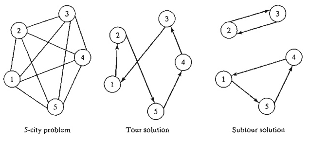
Figure 1 shows an example of a particular case of the traveller problem. The drawing on the left shows the network of cities (five cities) and their connections (from each city, in this case, it is possible to travel to any other city). The figure in the centre is a solution to the problem, i.e. an optimal route. Finally, the image on the right is an example of a sub-tour, which is ruled out by constraint 3.
| Constraint 3 admits formulations. In our case, we have applied the Dantzig-Fulkerson-Johnson formulation. In the blog of this link, different forms are explained and their efficiency is compared. |
In general, the standard form of a maximisation optimisation problem is  , where
  is the objective function, in contrast, a minimisation problem has the form
The modelling of a problem does not have to be unique. Sometimes, previous treatment of the data allows the model to be written in a simpler way. For example, the famous one-dimensional cutting problem is a paradigmatic case where the modelling of the problem gives rise either to a very computationally expensive problem or to a much simpler one.
In general, binary, integer or mixed-integer programming optimisation problems often explode heuristics and metaheuristics as well as stochastic methods making their complexity (solving time) increase considerably in function of the input data size compared to a linear programming problem. It is common to find cases where there are thousands of variables. In such cases, if one needs to recompute the optimal value within short time intervals since the data is regularly updated, the algorithm must be modelled so that the solution is quickly computed.
Problem Resolution
With the problem duly modelled, we can move on to the last step, problem-solving. Several characteristics, such as the type of variables, the constraints, the form of the objective function, etc., will determine the use of one or other solving techniques. These techniques must be known to exploit their strengths while considering their weaknesses (such as memory cost or execution time). The more complex libraries (see next point) can guide us in choosing such techniques, but depending on the case, such suggestions may not be optimal and may need to be modified by the user.
Modelling and Problem Solving with Libraries
In most cases, we will need computational help to solve the problem we are dealing with. For this purpose, there are several libraries in different programming languages. In this section, we will talk about some modelling libraries, some solving libraries and some libraries that combine functionalities and processes. However, we will underline that modelling and solving are two different concepts.

Modeller and Solver: Two Different Tools
To obtain the solution to an optimisation problem we need to model and solve it. These days there are tools in different programming languages that allow us to do one or both of these steps, but we must be relevantly aware of the difference between them.
On the one hand, modelling packages allow us to write a problem (parameters, variables, objective function and constraints) in a way that can be understood by the computer and by other packages. These, in general, high-level libraries, will allow us to abstract the problem, and facilitate its maintenance, exploitation, updating, etc.
However, to find the best solution (solve the problem) we need to apply a series of complex algorithms that depend (more or less) on the properties and characteristics of the given problem. Solvers take care of this. Solvers are a “toolbox” that, given a modelled problem, solves it in the best possible way. As there are many types of optimisation problems, there are solvers that are more or less complex, more or less ambitious, that allow us to solve more or less specific problems. When the problem has been mathematically formulated, it is interesting to think about which solver to use, bearing in mind its characteristics. If the problem is linear, the most appropriate choice is a solver that is prepared to solve this type of problem.
We can find libraries for modelling and problem-solving in different programming languages. Generally, the problem is modelled (translated) with a modelling library. Once the problem is modelled, the library calls a solver that takes care of applying the relevant algorithms to obtain the optimal. This architecture allows the flexibility to use different classes of solvers, allowing them to be adapted to the problem.
Finally, some solvers also allow the modelling of the problem. However, in these cases, the modelling is determined by, and therefore limited to, the solver in question.
Some Examples of Libraries
Nowadays, there are many different libraries, some paid and some free, that allow modelling and solving optimization problems. The choice of one or the other depends on the nature of the problem to be solved. It can be common to try different libraries (in general, solvers) during the development process to determine which one has the best performance for our particular problem.
These libraries are widely available for most commonly used programming languages, such as C++, Java or Python. Furthermore, more emerging languages focused on data analysis, such as Julia, also have ecosystems prepared to solve optimisation problems.
Several examples of the most commonly used libraries have been presented here.
Modelling Libraries
For modelling optimisation problems, some of the most commonly used libraries (but not the only ones) are:
- Pyomo: a free, open-source, high-level modelling language. It is a flexible, portable and maintainable framework. Allows calling a wide variety of solvers for linear and non-linear optimisation problems.
- PuLP: free and open source high-level library. Like Pyomo, it is flexible and portable. However, although it accepts different solvers, it is only intended for modelling linear optimisation problems.
- OR-Tools: Open optimisation software developed by google that can solve combinatorially, integer optimisation and linear programming problems. It accepts up to six commercial solvers like SCIP, GLPK, GLOP, CP-SAT, SCIP, GLPK, GLOP, CP-SAT and GLOP.
- AIMMS: algebraic modelling language that allows editing and creating graphical interfaces for models and a user-friendly interface. There are several solvers such as GUROBI, FICO, IPOPT… AIMMS supports linear, quadratic, integer-mixed, and stochastic optimisation problems.
- GAMS: high-level modelling system consisting of a compiler with several associated solvers. The compiler translates the problem into the appropriate language for the given solver.
- ILOG CPLEX: commercial software manufactured by IBM that allows modelling and solving optimisation problems. It also has a graphical interface to assist the user in modelling and reviewing the model and its results.
solvers
- Gurobi: one of the most widespread solvers, allows modelling and solving different types of problems (LP, MIP, Convex, Non-Convex, etc.). It can be used in a wide variety of programming languages, such as Java, Python, and C++.
- LocalSolver: solver specialised in combinatorial problems such as vehicle routing, \textit{scheduling} or \textit{supply chain} problems. Has APIS to be used in Python, Java, C# and C++.
- CBC: The COIN Branch and Cut solver (or CBC) is open source, written in C++, and inspired to solve integer-mixed programming problems.
- GLPK: stands for \textit{GNU Linear Programming Kit} aims to solve mainly linear programming and integer-mixed programming problems using several variables and parameters.
- IPOPT: Interior Point Optimizer is a Python package for solving large-scale non-linear optimisation problems.
Conclusions
In this article, we have seen the three fundamental pieces of an optimisation problem: the variables (the decision), what is to be optimised (the objective function) and the requirements (the constraints). In addition, we have discussed the importance of modelling the problem correctly and how different formulations can involve wide variations in time or memory when solving the problem.
We have also stressed the importance of correctly classifying the problem to apply the best algorithm for correct resolution and to be able to reduce the execution time and maximise its accuracy. Finally, we have presented different libraries that allow modelling and/or solving an optimisation problem.